Reversible Programming Primer: Basic Control Flow

In reversible programming languages, many of the fundamental concepts of control flow from traditional programming languages break down. All familiar forms of conditionals and looping allow for programs to effectively erase the history of their own operation, making it impossible to tell whether or not particular branches were taken to reach a particular result. In this third post on reversible programming, I will be going over the reversible counterparts of these control structures and showing how they can be used to implement some basic, familiar programming patterns.

A Disclaimer on Syntax

The code examples in this series use C-like imperative pseudocode. New reversible programming primitives will be given distinct syntax and keywords from the non-reversible primitives that they displace-- even if their functionality is nearly identical-- because the existing non-reversible primitives are still used throughout these posts to provide contrasting examples or to make the behavior of reversible primitives explicit by giving concrete implementations.

This syntax is also distinct from the syntax of existing reversible programming languages, which often choose to reuse the syntax and keywords of non-reversible programming languages for corresponding-but-not-equivalent concepts.

The Problem with Control Flow in Reversible Programming Languages

The core constraint of reversible computing is that erasing information is not allowed. For example, we are not allowed to destructively assign a new value to a variable:

x = 0;
// This erases the previous value of `x` and replaces it with `0`.

However, even if we only use reversible operations, if we use non-reversible control flow, we can still implement non-reversible behavior. For example, we can implement the above non-reversible assignment statement using a reversible compound assignment and a while loop:

x = 0;

// Is equivalent to:

while(x != 0) {
  x @- 1;
}

The @- here is the “in-place” syntax introduced in the previous post in this series applied to subtraction. I would recommend reading the previous posts if you haven’t already, so that you will be familiar with the new syntax that has already been introduced.

Since this structure implements a non-reversible assignment, some part of it must be non-reversible. Subtracting 1 from an integer is reversible, and conditions can be evaluated reversibly. So, it must be that the while loop itself is non-reversible somehow.

Generally speaking, if the condition is initially false, you skip the while loop entirely. If the condition is initially true, you enter the loop and repeat the body until the condition becomes false, at which point you exit the loop. Even though the condition determines which path you take, by the time you arrive the other side of the while loop, the condition can only have one possible value-- false-- meaning that the while loop itself erases the information that you would need to determine whether or not it ever executed.

This is a problem with virtually all traditional forms of control flow. They either require or allow for conditionally-executed code to modify the state that was used to decide if that code should run, and allow this to happen in a way that obscures the history of the program’s execution.

We will need to rethink how control flow is structured in order to be able to perform the sorts of loops and conditionals that we are used to without breaking reversibility.

between

The between loop is the fundamental looping control structure for reversible programming languages. Conveniently, it’s possible to implement a between loop in terms of regular non-reversible control structures:

between(condition) {
  // body
}

// is equivalent to:

if(condition) {
  do {
    // body
  } while(!condition);
}
// here, the two instances of `condition` represent two copies of the exact same boolean expression.

Even if you are a programmer and are familiar with do/while, it might be difficult to pick apart how this code works, as it is very unusual. The basic behavior can be summarized as follows:

• If condition is initially false, skip the loop entirely.
• If condition is initially true, repeatedly execute the block until the condition is true again after executing the block. Then exit the loop.

To put it more concisely, “enter if true, exit if true”.

This differs from a standard non-reversible while loop, which would be “enter if true, exit if false”.

This behavior is unintuitive from a programming perspective, and doesn’t match the behavior of most real world systems either. But there is one kind of real world system that can model reversible control flow really well: trains.

This is a simplified animation of what’s called a “double crossover turnout”. A double crossover turnout is a section of track that can allow train cars to switch between two parallel tracks. If we were to take one of those two parallel tracks and join the ends into a loop:

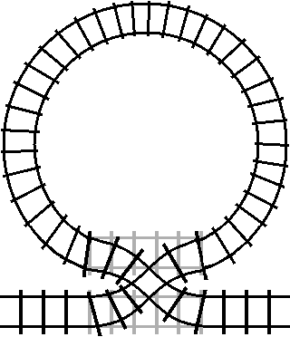
We get the railroad equivalent of a between statement. The loop of track is a stand-in for the body of the between loop. You can see that when the track is not switched (the condition is false), the train will bypass the loop without entering it:

The train will only enter the loop when the track is switched (the condition is true) However, once the train has entered the loop, the train will exit the loop the next time it passes the crossover while the crossover is switched (the condition is true again).

If you want to remain in the loop, you need to switch the track after you enter it. It might seem sufficient to just toggle the condition directly:

bool condition <- true;
between(condition) {
  !@condition;
}

However, since you’re in a loop, you would just end up toggling the condition again on the second iteration, and accidentally escaping the loop. You need to find a way of changing your looping condition in a way that will not immediately flip back. One crude method might be to use the modulo operator.

int i <- 0;
between(i % 10 == 0) {
  printline(i);
  i @+ 1;
}

This would print the numbers 0, 1, 2, 3, 4, 5, 6, 7, 8, and 9.

However, this is clearly not ideal for most situations, and that’s likely the reason that this particular kind of loop has not been included in most reversible programming languages despite being so simple and fundamental. However, I’ve found that the between loop serves as a terrific foundation, and the remainder of this post will use the between loop as a building block for implementing more convenient forms of control flow.

given

Normal if statements have similar issues to loops. Given the following code:

if(x == 1) {
  x @- 1;
}

If x is 0 following the conditional, it is impossible to tell if it was initially 0 and skipped the conditional or if it was initially 1 and was modified by the inner subtraction. We need an alternative conditional statement designed to prevent this from happening.

So, we can introduce the “given statement” (as in, “given some condition, perform some action”):

given(condition) {
  // body
}

// Is equivalent to:

if(condition) {
  assert(condition);

  // body

  assert(condition);
}

Here, the given statement asserts that the condition has not changed before exiting the body. As long as the condition remains the same, we will always be able to backtrack through the given statement by using the same condition to decide whether or not to enter it while stepping through the code in reverse.

As described in the disclaimer, given is intentionally given a different name from normal if statements in this series of posts for clarity; however, I don’t think there’s any practical issues with calling a reversible conditional an “if statement” in a real reversible programming language (the same is not true for “reversible while” loops; see the extra section on between loops for the argument there).

The given statement can also be written directly in terms of between:

given(condition) {
  // body
}

// Is equivalent to:

between(condition) {
  assert(condition);

  // body

  assert(condition);
}

Since we assert the condition at the end of the body, the “loop” is guaranteed to terminate after a single iteration (or raise an error).

A given statement behaves exactly the same as an if statement if the body of the given statement does not modify any variables used to compute the condition. For example, if we are doing conditional printing.

printline("Select an option:");
printline("1. Rock");
printline("2. Paper");
printline("3. Scissors");

string response <- readline();

given(response == "1") {
  printline("The computer chose paper; you lose");
}
given(response == "2") {
  printline("The computer chose scissors; you lose");
}
given(response == "3") {
  printline("Sorry kid, but the house always wins. The computer chose rock.");
}

The bodies of these given statements do not mutate any variables, so they are easy to work with.

However, the restriction of not changing any variables used to compute the condition can be a little inconvenient in some circumstances. Consider something as simple as wanting to set an integer to 10 if its previous value was 5:

int value <- 5;

given(value == 5) {
  value -> 5;
  value <- 10;

  // ERROR: value no longer equals `5`.
}

There are various workarounds for this:

int value <- 5;

given(value == 5 ^ value == 10) {
  value -> 5;
  value <- 10;
}

// Or:

int value <- 5;

bool activateConditional <- value == 5;
given(activateConditional) {
  value -> 5;
  value <- 10;
}
activateConditional -> value == 10;

However, both of these are clunky and have their own quirks. Let’s continue to look at some variations on given statements, but keep these problems in the back of your mind, because we’ll circle back around to a more general fix for some of the clunkiness of both given and between statements.

given/else

It’s common for conditional statements to have an alternative else block that is executed if the condition is false, and given statements support else in basically the way you would expect.

given(condition) {
  // true-body
} else {
  // false-body
}

// Is equivalent to:

if(condition) {
  assert(condition)

  // true-body

  assert(condition)
} else {
  assert(!condition)

  // false-body

  assert(!condition)
}

Just as the true case asserts that the condition remains true after its block is executed, the false case must assert that the condition remains false. In fact, because these mutually-exclusive conditions are maintained before and after each block, we can actually implement given/else as just a sequence of two separate given statements:

given(condition) {
  // true-body
} else {
  // false-body
}

// Is equivalent to:

given(condition) {
  // true-body
}
given(!condition) {
  // false-body
}

given/else can be used for many of the same purposes as a normal if/else statement, but with the added limitations that come along with given statements. But, they are more than sufficient for common cases of picking one of two alternative actions based on a condition, as long as the action doesn’t modify the condition, such as a simple case of selecting the largest of two numbers:

int a <- some_value;
int b <- some_other_value;

int max;
given(a > b) {
  max <- a;
} else {
  max <- b;
}

“else given”

Programming languages often allow for a compound else if for long chains of if statements with decreasing priority.

if(x <= 1) {
  // do something
} else if (y <= 5) {
  // do something
} else if (z <= 10) {
  // do something
} else {
  // do something
}

Since each if statement is only evaluated if the previous if statement’s condition was false, it implicitly includes the negation of all previous if statements’ conditions in its condition. The if statement above could be written equivalently as:

if(x <= 1) {
  // do something
} else if (x > 1 && y <= 5) {
  // do something
} else if (x > 1 && y > 5 && z <= 10) {
  // do something
} else if(x > 1 && y > 5 && z > 10) {
  // do something
}

The semantics of the given version of this structure become more obvious when you consider that else if is really just “syntactic sugar” for an if statement nested inside of the else statement of another if statement:

if(x <= 1) {
  // do something
} else {
  if (y <= 5) {
    // do something
  } else {
    if (z <= 10) {
      // do something
    } else {
      // do something
    }
  }
}

This same structure can be reproduced with reversible given/else statements:

given(x <= 1) {
  // do something
} else {
  given (y <= 5) {
    // do something
  } else {
    given (z <= 10) {
      // do something
    } else {
      // do something
    }
  }
}

However, this kind of nesting of conditionals requires extra care in reversible programming languages that might be non-obvious, and might be especially non-obvious when nesting conditionals in else blocks. Remember that when we exit a given statement, we assert that the condition of that given statement has not changed. This means that we must be careful within the body of deeply nested given statements, to avoid changing, not just the condition of that given statement, but also all of the parent statements.

For example, imagine that we inserted the following code into the z <= 10 case:

int x <- 2;
int y <- 6;
int z <- 9;

given(x <= 1) {
  // do something
} else {
  given (y <= 5) {
    // do something
  } else {
    given (z <= 10) {
      y @- 5;
    } else {
      // do something
    }

    // ERROR: y is no longer greater than 5.
  }
}

Here, the content of our z <= 10 block does not modify its own condition’s truth value, but it does modify the parent block’s y <= 5 condition’s truth value. By subtracting 5 from y, which is initially 6, y <= 5 flips from being false to true. This causes a runtime error when that parent block asserts that its condition hasn’t changed.

This kind of nesting requires a greater level of attention to detail, but there’s no reason that we can’t provide the equivalent syntactic sugar for given/else for anyone who wants to use it:

given(x <= 1) {
  // do something
} else given (y <= 5) {
  // do something
} else given (z <= 10) {
  // do something
} else {
  // do something
}

Diodes

There are a number of inconvenient things about the control structures that we’ve examined so far. The fact that the condition of a given statement must remain true when it exits makes it hard to do anything useful inside of a conditional statement. On the other hand, the looping behavior of the between loop is very difficult to reason about; behavior that starts and stops on the same condition is confusing and doesn’t match many common patterns in computer programs or the real world.

In both cases what we’d really like is the ability to express that we “enter” a control structure under one condition, and we “exit” the control structure under a different condition.

So, let’s imagine a new logical data type: a Diode. A Diode represents a pair of conditions that must become true in a particular order. We could define a Diode like this:

struct Diode {
  bool entry_condition;
  bool exit_condition;
}

We can construct a Diode by joining two conditions with a thick right arrow operator (=>).

entry_condition => exit_condition

=> could be referred to as the “before” operator, as in “entry_condition before exit_condition”.

Diodes give us an intuitive syntax to express that a control structure has separate entry and exit conditions. Let’s look at some examples of new control structures that use Diodes to address the limitations of the previous boolean-based control structures.

Diode-Based for

Writing loops with a shared entry and exit condition was a major pain point, so introducing a new type of loop that uses Diodes to specify those conditions separately should make looping a lot easier. We can implement a new Diode-based loop in terms of the existing boolean-based between loop as follows:

for(entry_condition => exit_condition) {
  // body
}

// is equivalent to:

between(entry_condition ^ exit_condition) {
  assert(!exit_condition);

  // body

  assert(!entry_condition);
}

Here, we skip the loop if both conditions are false or both conditions are true. If only the exit_condition is true, then we raise an error-- that’s the “conditions must become true in a particular order” rule. But, if only the entry_condition is true, then we enter the loop.

Once in the loop, we exit at the end of the loop if only the exit_condition is true (mirroring the entry rule). If the entry_condition is true at the end of the loop, we raise an error, regardless of if the exit_condition is true. If neither are true, then we repeat the loop.

I’ve used the keyword for here, which overlaps with the looping keyword in non-reversible programming languages that is traditionally used for looping over sequences or ranges of numbers. The use of the before operator (=>) should make it clear whether a given for loop in the code examples is a traditional non-reversible for loop or the new reversible version. But, in this case, I think a shared name makes sense, because they are really used for very similar types of code and for loops have many different variations even within non-reversible programming languages. Loops equivalent to traditional for loops can be rewritten with this new control structure in a straightforward way:

for(int i = 0; i < count; i++) {
  // body
}

// is equivalent to:

int i <- 0;
for(i == 0 => i == count) {
  // body

  i @+ 1;
}
i -> count;

Since we skip the loop if both conditions are true, the loop here will be skipped when the count is 0, lining up with our expectations. At long last, we can update our “FizzBuzz” implementations for the 21st century:

int i <- 1;
for(i == 1 => i == 101) {
  given(i % 3 == 0) {
    print("Fizz");
  }
  given(i % 5 == 0) {
    print("Buzz");
  }
  given(i % 3 != 0 && i % 5 != 0) {
    print(i);
  }

  printline();
  i @+ 1;
}
i -> 101;

In practice, Diode-based for loops are almost always preferable over between loops except in cases of very specific optimizations where there’s a lot of redundancy between the entry_condition and exit_condition. However, having between loops as a primitive for building other control structures is very valuable for understanding how reversible programming as a whole works.

Diode-Based given

With boolean-based given, we had some difficulty with writing conditional statements that modify the variables that determine the conditions for their own execution. Diode-based given statements can simplify these conditionals fairly substantially.

given(entry_condition => exit_condition) {
  // body
}

// Is equivalent to:

between(entry_condition || exit_condition) {
  assert(entry_condition);

  // body

  assert(exit_condition);
}

Fittingly, in the case where the entry_condition and exit_condition are the same, this reduces to our original single-condition given statement.

A Diode-based given statement allows us to alter some of the variables that determine our conditions without causing an error. One simple use case for this would be resizing the backing array for a dynamically-sized list:

given(list.count == list.capacity => list.count * 2 == list.capacity) {
  int new_capacity <- list.capacity * 2;
  T[] new_backing_array <- new T[new_capacity];

  // Here, we are looping over all of the indices of the current backing array
  // and `swap`ing its values into the new backing array.
  int i <- 0;
  for(i == 0 => i == list.capacity) {
    new_backing_array[i] >-< list.backing_array[i];
    i @+ 1;
  }
  i -> list.capacity;

  new_capacity >-< list.capacity;
  new_backing_array >-< list.backing_array;

  // here, `uncopy`ing a "new" array is used as a syntax for deallocating an
  // array and clearing the variable storing it, as this is the exact inverse
  // of the `copy` version.
  new_backing_array -> new T[new_capacity];
  new_capacity -> list.capacity / 2;
}

Here our entry condition is that the list is full, and our exit condition is that the list is exactly half-full. Since we double the size of the list if it’s full, the exit condition will always be successfully reached when the entry condition is initially true.

It’s often useful to be able to verbalize code, so it might be useful to read this structure as: “given entry_condition before exit_condition”. In this case, “given the list’s count equals its capacity before the list’s count times two equals its capacity”.

Diode-Based given/else

A Diode-based given/else statement can be defined analogously. If the entry_condition is not met, then the else block will be executed instead; however, the else block must assert that the exit_condition is not met when it exits (since the exit_condition will be met when the given block exits).

given(entry_condition => exit_condition) {
  // true case
} else {
  // false case
}

// Is equivalent to:

bool condition <- entry_condition;
given(condition) {
  condition -> entry_condition;

  // true case

  condition <- exit_condition;
} else {
  condition -> entry_condition;

  // false case

  condition <- exit_condition;
}
condition -> exit_condition;

Here, condition is a temporary variable, and because of the order of initializations and uninitializations, it will always be properly cleared when the statement finishes.

This structure actually hints at some of the details of how expressions are evaluated in reversible programming languages, but I will go into more detail on expression evaluation in a future post.

And, of course, because else given is just syntactic sugar for nested given/else statements, we can have given/else chains, and even include a mixture of boolean and Diode-based conditions:

given(x <= 1) {
  // do something
} else given (x <= 5 => x > 5) {
  // do something
} else given (x <= 10) {
  // do something
} else {
  // do something
}

Wrapping Up

With the introduction of basic control flow, we are official in the territory of being able to write practical algorithms in reversible programming languages. We have managed to define all of our primitives so far in terms of three reversible primitives: bitwise XOR compound assignment, assertions and the between loop.

The next post in this series will begin to explore some control structures that are only available in the world of reversible programming, which serve unique functions that are inconceivable in the world of non-reversible programming. One such control structure will prove to be even more fundamental than looping, and will displace the between loop as our third basic primitive. Up until this point, reversibility has largely been a restriction, but this will finally start to get into some of the new capabilities that reversibility grants to computer programs.

Extra: Infinite Loops & “Entropy Complexity”

It’s very common-- especially user-facing software-- for a program to enter into an “infinite loop”, in which it repeatedly presents its user interface to the user. However, reversible programming languages encounter some unique problems with the concept of infinite loops.

Let’s just imagine that we had some sort of magical construct for looping indefinitely, called loop:

loop {
  printline("Looping Forever!");
}

In a reversible programming language, it must always be possible to “rewind” the execution of the program to any previous state. With this looping construct, we enter the loop unconditionally and then never exit; but since there was no specific condition that was met to mark our entry to the loop, how would we know how many times we should loop backwards before exiting the loop when we rewind the program? The answer is: there is no way to know, and consequently, unconditionally entering an infinite loop erases information, which is not allowed in a reversible program.

The simplest-- and often most-efficient-- method to work around this is to literally count the number of times that we have repeated the loop. When we rewind, we can then count backwards to make sure that we loop backwards the correct number of times before exiting. For example, we can count the number of iterations of our loop as follows:

int i <- 0;
between(i == 0) {
  printline("Looping Forever!");

  i @+ 1;
}

printline("Whoops, only looped 4,294,967,296 times!");

However, even this implementation has a problem: the basic integer types of most programming languages have a limited range, after which, they wrap around and return to being 0. If int is a 32-bit integer, then that means that this “infinite” loop would be executed exactly 4,294,967,296 times before exiting. To get a truly infinite loop, we need an arbitrary-precision integer, colloquially known as a “big integer”, which is a special data type that dynamically allocates more memory to represent arbitrarily large numbers.

BigInteger i <- 0;
between(i == 0) {
  printline("Looping Forever!");

  i @+ 1;
}

Big integers can represent arbitrarily large numbers, but this comes with the downside that they must allocate memory on the heap to store those numbers, and must allocate more memory the larger the number gets. So, as our counter grows, it will gradually take up more and more memory.

In computer science, it’s common to talk about the “time” and “space” requirements for certain computational tasks. “Time complexity” refers to the running time of an algorithm and the way in which that grows as a function of some parameter of the algorithm. “Space complexity” refers to the amount of temporary memory or “scratch space” that is needed to hold temporary data during the algorithm’s execution, and the way in which that grows as a function of some parameter of the algorithm.

This infinite loop is the first instance so far of a sort of unique computational resource requirement for reversible computation: the amount of memory that must be rendered (semi-)permanently unusable by the algorithm for the entire duration that the result of the algorithm is being used, and the way in which that grows as a function of some parameter of the algorithm.

The classic example here is sorting a list. Sorting a list inherently destroys the information about the order that the list was originally in, so a reversible sorting function must preserve that information somewhere. A common solution is to output an array of integers storing the original order of the list as a permutation array. This permutation array is the “(semi-)permanently unusable” memory generated by the sort. There is no way to get rid of it, except by rolling back the sort and unsorting the list.

This information is effectively random and meaningless from the program’s perspective, analogous to the information theory notion of “entropy” as uncertainty about the value of variables. This information also cannot be uncomputed without rolling back the algorithm that produced it, and would otherwise need to be erased to clean up the program’s memory, which-- as discussed in the introduction to the series-- would generate thermodynamic entropy; so, you could think of this data as “potential thermodynamic entropy”. As a result, I like to think of this as the “entropy complexity” of an algorithm. “Entropy” feels like it fits right in along side “time” and “space”.

In the case of our infinite loop, the big integer counter is a piece of this “potential entropy”: its value is entirely meaningless to the program, but we need it to be able to write the loop in a reversible way. Because every bit added to an integer doubles the number of possible values that integer can assume, our example infinite loop here would have “logarithmic entropy complexity”: the amount of memory rendered (semi-)permanently unusable is proportional to the logarithm of the number of iterations of the loop.

Extra: The Lack of continue and break

Non-reversible programming languages generally feature continue and break statements as convenience methods for controlling loops. A typical pattern for continue might be something like:

while(condition) {
  do_some_work();

  if(other_condition) continue;

  do_some_more_work();
}

Here, if the continue statement is executed, then the remainder of the loop is skipped. This can be useful, for example, if you are searching a collection and have already determined that the current item in the search cannot be what you are looking for; there’s no reason the continue applying the remaining checks to that item, so you might as well continue and skip to the next item.

continue statements themselves would be complicated to reason about as elements of a reversible program, because, since you can continue out of the final iteration of a loop, they essentially represent an extra entry location for the loop that can only be accessed while running code backwards, and that has complex conditions associated with jumping to it.

We can get the majority of the benefit of continue statements without the complication in an obvious but somewhat less flexible form:

for(entry_condition => exit_condition) {
  do_some_work();

  given(!other_condition) {
    do_some_more_work();
  }
}

You can simply invert the condition and make the remainder of the work conditional rather than making the continue conditional. This is a more classic pattern that is generally avoided in modern programming because it leads to deep nesting, but it preserves the basic functionality of continue statements for reversible programs, without needing to introduce features that make backtracking excessively difficult to follow.

break statements are even more difficult to reconcile with reversible programming languages. A typical pattern for break might be something like:

while(condition) {
  do_some_work();

  if(other_condition) break;

  do_some_more_work();
}

Here, if the break statement is executed, the remainder of the loop is skipped, and the entire loop terminates prematurely, immediately jumping to the code following the loop. This is commonly-used when it’s possible to determine that there is no more useful work to be done-- not just in the current iteration of a loop, but in all of the remaining iterations of the loop-- so you should stop looping entirely.

Another common pattern is to make the loop unconditional, and then use break statements as the only method of exiting the loop.

while(true) {
  do_some_work();

  if(other_condition) break;

  do_some_more_work();
}

In either case, break statements introduce similar conceptual complications to continue statements, because they introduce additional entry points for the loop body during backtracking. We can approximate a break statement by using the same pattern as the continue statement simulation to skip the remainder of the body, and then use a temporary variable to control the early loop termination:

bool should_break <- false;
between(condition || should_break) {
  do_some_work();

  given(other_condition) { !@should_break; }
  if(!should_break) {
    do_some_more_work();
  }
}
should_break -> other_condition;

However, this simulated break statement comes with a few big caveats:

• The other_condition must be a condition that it is actually possible to uncompute outside of the loop.
• The loop will not terminate in a predictable state, so it may be very difficult to clean up any other variables used to control the loop.

So, this is not exactly an ideal solution.

But, of course, as is always the case, reversible programming both causes the problem and provides the solution. In the next post in the series, which covers backtracking, I will be introducing a supercharged version of Lecerf-Bennett reversal, which can serve many of the normal functions of break statements in a more idiomatically-reversible way.

Extra: The Name of the between Loop

The between loop is usually called a “reversible while loop” in the rare instances where it comes up in discussions of reversible programming languages. However, calling this a while loop seems more likely to confuse people than it is to be helpful.

Generally speaking, the names of control structures map onto words that have a similar function in the English language, meaning that reading code aloud generally sounds like a coherent-if-stilted list of instructions. Looking at code like:

int sum = 0;
while(list.count > 0) {
  sum += list.pop();
}

This code can be verbalized as “while the count of items in the list is greater than zero, pop the next item off the list and add it into the sum.”

However, “while” does not map semantically onto the behavior of the between loop. “While” means “for as long as the condition is true”-- which means it should stop when the condition becomes false. However, between stops when its condition becomes true. We could negate the condition of the between loop, which would leave us with a loop that exits when its condition becomes false; however, this would mean that the loop would only be entered when the condition was initially false, which doesn’t agree with how “while” works grammatically either.

We can actually break down all of the cases of loops that are entered and exited on different combinations of truth values of the loop condition:

Neither of the reversible cases are compatible with commonly-used names of looping control structures.

Additionally, unlike some control structures we will examine in future posts, between loops could exist without issue in normal, non-reversible programming languages-- an explicit implementation in terms of if statements and do/while loops was given earlier in this post-- so I think it makes sense to give between statements a different syntax than while loops so that the control structures could coexist.

Extra: Alternative for Loop Definition

There is one behavior of the Diode-based for loop that I think is arguably not really justified by my prior explanation. To lay out the for loop’s behavior again:

1. If only the entry_condition is met when a for loop is encountered, you enter the loop.
2. If only the exit_condition is met at the end of the block, you exit the loop.
3. If only the exit_condition is met when a for loop is encountered, an error is raised.
4. If only the entry_condition is met at the end of the block, an error is raised.
5. If neither condition is met when a for loop is encountered, you do not enter the loop and skip it instead.
6. If neither condition is met at the end of the block, you do not exit the loop and repeat it instead.
7. If both conditions are met when a for loop is encountered, you do not enter the loop and skip it instead.
8. If both conditions are met at the end of the block, an error is raised.

There’s very strong inside/outside and forward/backward symmetry of these rules, with one glaring exception in 7 and 8: both conditions being true only raises an error when it occurs inside of the loop.

We could imagine an “alternative” for loop where the 8th rule was instead:

If both conditions are met at the end of the block, you do not exit the loop and repeat it instead.

We could implement such an alternative foralt loop as follows:

foralt(entry_condition => exit_condition) {
  // body
}

// Is equivalent to:

between(entry_condition ^ exit_condition) {
  assert(entry_condition || !exit_condition);

  // body

  assert(exit_condition || !entry_condition);
}

As discussed earlier in the post, for is most-commonly used for code that iterates through a collection like this:

int i <- 0;
for(i == 0 => i == list.count) {
  do_something_with_list_item(list[i]);
  i @+ 1;
}
i -> list.count;

If we substitute our new foralt, the code functions in exactly the same way.

int i <- 0;
foralt(i == 0 => i == list.count) {
  do_something_with_list_item(list[i]);
  i @+ 1;
}
i -> list.count;

This makes sense, because the inner error condition was not triggered in the first example, so the extra inner looping condition would not be triggered in the second example. So, there’s this one common case where they happen to behave the same. However, this seems to actually be the rule, rather than the exception. I have not yet found a single example of a practical application in which the choice between these two control structures would affect the behavior of any program, or where you would have to write code differently depending on which one you picked.

It would seem like the more symmetrical control structure should be favored then. However, if we go out of our way to construct a contrived example that does exercise the difference in behavior, the problem with foralt becomes more clear.

Consider the following code:

int i <- 0;
int j <- 10;

foralt(i < 10 => j < 10) {
  i @+ 1;
  j @- 1;
}

Take a moment to try to figure out what the value of j will be when this code finishes executing.

Our entry_condition is that i < 10, which is initially true and our exit_condition is that j < 10, which is initially false. So, we will enter the loop.

Within the loop body, we increment i, so it must eventually become greater than 10, and we decrement j, so it must eventually become less than 10. But, what will the value of j be when the loop finally exits?

The j < 10 exit_condition, coupled with the fact that j is decremented by 1 in each iteration of the loop might suggest that the answer is 9, which would be the first value of j that satisfies the exit_condition. However, the correct answer is 0. Even after the exit_condition becomes met, the loop must continue until the entry_condition is not also met, which will take 10 iterations of the loop.

This is deeply unintuitive, because it means that the exit_condition doesn’t meaningfully define the “trigger” that causes the loop to exit, and generally makes it harder to reason about the behavior of the foralt loop when it’s possible for the entry_condition and exit_condition to overlap.

This is why the definition chosen for the Diode-based for loop makes this case an error instead of a continuation of the loop. However, this is simply one contrived example I’ve managed to put together. It might turn out that there are actually useful consequences of foralt’s behavior in certain circumstances that I just haven’t encountered yet. For the time being, the correct approach might be to consider this case to be “undefined behavior” until a definitive decision can be reached one way or the other.