Reversible Programming Primer: Backtracking Control Flow
So far in this series, reversible computation has introduced a lot of restrictions on how you can write code. However, reversible programs are also capable of some very unique functionality that is simply impossible without imposing the constraint of reversibility. In this fourth post on reversible programming, we will finally be justifying the name “reversible computing” by exploring how reversible programming languages can allow programmers to “run code in reverse” and all of the unique things this feature allows you to accomplish.
A Disclaimer on Syntax
The code examples in this series use C-like imperative pseudocode. New reversible programming primitives will be given distinct syntax and keywords from the non-reversible primitives that they displace-- even if their functionality is nearly identical-- because the existing non-reversible primitives are still used throughout these posts to provide contrasting examples or to make the behavior of reversible primitives explicit by giving concrete implementations.
This syntax is also distinct from the syntax of existing reversible programming languages, which often choose to reuse the syntax and keywords of non-reversible programming languages for corresponding-but-not-equivalent concepts.
undo
Let’s start off with the most direct possible method of running code in reverse,
which you could call an undo statement.
undo {
  // body
}
Whereas given executes a block of conditionally, and between executes a
block of code in a loop, undo executes a block of code “in reverse”. When code
is “executing in reverse”, the program executes the reversed version of each
statement in reverse order.
For example, consider the following code:
int a <- 1;
int b <- 1;

// Executes first:
//   `a` becomes 1 + 1 = 2
a @+ b;
// Executes second:
//   `b` becomes 1 + 2 = 3
b @+ a;

printline("a = {}, b = {}", a, b);
// prints "a = 2, b = 3"
This is just some fairly simple arithmetic. But, let’s wrap those in-place
arithmetic operations in an undo block.
int a <- 1;
int b <- 1;

undo {
  // Executes second:
  //   The inverse of `a @+ b` is `a @- b`.
  //   `a` becomes 1 - 0 = 1
  // Second:
  a @+ b;

  // Executes first:
  //   The inverse of `b @+ a` is `b @- a`.
  //   `b` becomes 1 - 1 = 0
  b @+ a;
}

printline("a = {}, b = {}", a, b);
// prints "a = 1, b = 0"
Since the block executes in-reverse, we end up with a totally different result.
But, the real utility of undo becomes more obvious if we run some code and
then immediately undo the same code:
int a <- 1;
int b <- 1;

a @+ b;
b @+ a;

undo {
  a @+ b;
  b @+ a;
}

printline("a = {}, b = {}", a, b);
What would you imagine that this program prints?
The answer is: "a = 1, b = 1". True to its name, running the same code
in reverse with undo “undoes” the result of applying it forward.
This core capability to “run code in reverse” is the foundation of the unique
capabilities of reversible programming languages. Plain undo statements are
not likely to be used frequently on their own, but they make up half of the
behavior of one of the most mind-bending control structures in reversible
programming languages: the turn statement.
turn
A turn statement is kind of like a conditional undo statement. If the
condition is true, it behaves exactly like an undo statement:
turn(true) {
  // body
}

// Is equivalent to:

undo {
  // body
}
And when the condition is false, the body is just executed as-is with no
change in behavior:
turn(false) {
  // body
}

// Is equivalent to:

// body
Just for parity, we can treat this as a kind of “do statement” that just
executes a block of code in its own scope:
turn(false) {
  // body
}

// Is equivalent to:
do {
  // body
}

// Both equivalent to:

// body
So far so good. However, this is only what happens if the condition does not
change while the turn statement is executing. What happens if the condition
changes?
As with the previous post,
it’s easiest to illustrate the behavior with a railway analogy. Last time, we
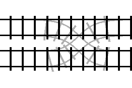
discussed how the structure of a between loop corresponded to the structure of
a double crossover turnout:
However, it turns out that turn statements also correspond to double
crossover turnouts, just with the “loop” bridging a different set of tracks.
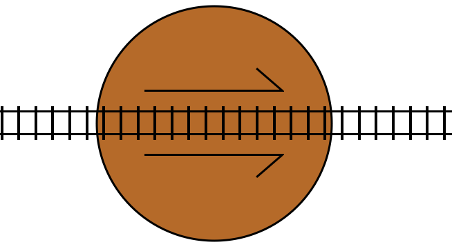
For reference, the between loop railway loop was represented like this:
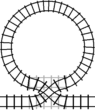
If we instead connect the two outputs on one side of the turnout together in a
loop, then we get a turn statement:

Here, the arrow is indicating the “forward” direction of the track inside the loop.
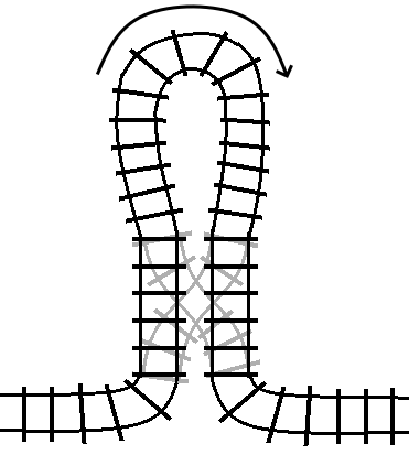
If the track is not switched (the condition is false), then the train travels
through the loop in its forward direction, and then proceeds on to the track
following the turn statement, just like a do statement:
If the track is switched (the condition is true), then the train travels
through the loop in its reverse direction, and then proceeds on to the track
following the turn statement, just like an undo statement:
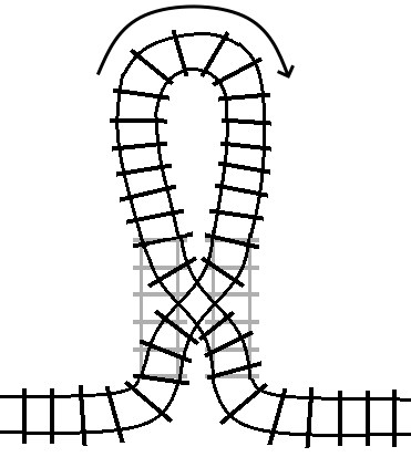
If the condition changes while we are inside the block, that is the equivalent of the track switching while we are on the loop of track. So, what happens…?

We exit the turn statement traveling in the opposite direction that we
initially entered it. In other words, the “turn” statement not only allows us
to execute code in reverse, it also allows us to “turn” around and start
traveling backwards through the code that we were executing before the turn
statement.
The fact that turn statements and between loops can be represented by the
same underlying track switching mechanism gives them a really interesting sort
of duality. However, for turn statements specifically, there’s actually an
even simpler railway analogy that makes their behavior even more obvious:
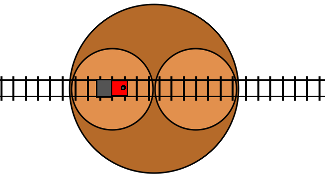
turn statements are like turntables.

This is a railway turntable representing a turn statement. If the condition
for the turn statement is true, then it rotates by 180 degrees. The arrow
markers indicate the “forward” direction of the track in the turntable.
If the track is not switched (the condition is false), then the train travels
through the turntable track in its forward direction, and then proceeds on to
the track following the turn statement, just like a do statement:

If the track is switched (the condition is true), then the train travels
through the turntable track in its reverse direction, and then proceeds on to
the track following the turn statement, just like an undo statement:

And, just as with the double crossover representation, switching the tracks while the train is on the turntable will result in the train turning around and exiting the turntable in the opposite direction.
The applications of this may not be immediately obvious-- it’s fairly alien to any ordinary understanding of control flow. However, it turns out that the ability “turn around” and start executing code in reverse is an extremely powerful programming primitive with a number of applications.
Toggle Reflectors and Backtracking
The most immediately obviously new possibility for control flow is: backtracking.
Consider the following code:
turn(some_boolean) {
  !@some_boolean
}
Regardless of the direction the code is executing or the initial value of
some_boolean, this code has the effect of:
- Toggling
some_boolean. - Reversing the direction of execution.
We could call this structure a “toggle reflector”, since it toggles a variable, and “reflects” the instruction pointer, sending it traveling in the opposite direction through the program. This is a very useful building block for doing a variety of forms of reversible control flow.
These toggle reflectors can be used as a primitive to initiate or terminate
backtracking. For example, we can use turn statements to implement a basic
error-handling system that rolls back work when an error occurs:
bool error_encountered <- false;
bool handling_error <- false;

// On our first pass, this `given` statement will be skipped.
given(error_encountered) {
  // This toggle reflector terminates the backtracking
  // initiated by the error condition later in the program
  // and sets the `handling_error` flag.
  turn(handling_error) {
    !@handling_error;
  }
}

// Pre-backtracking we enter the `do_some_work` block.
// Post-backtracking, we enter the `handle_error` block.
given(!handling_error) {
  do_some_work();

  // Whoops, we encountered an error-- let's set the
  // `error_encountered` flag and initiate backtracking.
  given(some_error_condition) {
    turn(error_encountered) {
      !@error_encountered;
    }
  }
} else {
  handle_error();
}
When we run this program, initially the given(error_encountered) block will
be skipped, and we will enter the work branch of the second given statement.
Following the completion of do_some_work(), we check for an error and use a
toggle reflector to initiate backtracking if an error occurred, setting the
error_encountered flag to indicate to the error-handling code that an error
occurred.
During backtracking all of the work from do some work() is rolled back as
control flow backtracks through that code. Control flow now enters the
given(error_encountered) statement that was skipped initially, and this
terminates the backtracking and sets the handling_error boolean. This causes
the given/else statement to choose the error-handling branch instead of the
work branch.
A fully-featured error-handling system would likely also want to provide a way to dispose of the boolean values here, since their values cannot be reliably uncomputed, so they would otherwise become junk data. But a sketch of a more robust error-handling system for reversible programming languages will be the subject of a future post.
This primitive capability for backtracking turns out to be useful in
implementing more complex forms of control flow, and by developing a strong
understanding of how turn statements work, it will be easier to understand
some of the additional control structures that will be introduced in this and
later posts. However, in addition to being useful for defining very complex
control structures, turn statements can also be used to implement other
extremely fundamental control structures.
Fundamentality
turn statements turn out to be very fundamental-- even more fundamental than
loops or conditionals, because they can be used to implement loops and
conditionals.
We can actually implement between in terms of turn and a temporary variable,
toggle, as follows:
between(condition) {
  // body
}

// Is equivalent to:

bool toggle <- true
turn(condition ^ toggle) {
  turn(condition ^ toggle) {
    !@toggle;

    // body
  }

  turn(condition ^ toggle) {
    !@toggle;
  }
}
Here, all three turn statements have the exact same condition, so all three
blocks are inverted together. But since the two inner turn statements are
inside of the third turn statement, they get inverted once by the outer turn
statement, and then invert themselves. This means that the absolute
“orientation” of the inner turn statements always remains the same. Toggling
the condition just causes them to “switch places”.
With the turntable analogy, there’s an easy-to-understand visual metaphor for how the loop occurs:
Here we have two turntables nested on a larger turntable, just as we have two
turn statements nested in an outer turn statement in the code. When we
toggle the toggle variable, this results in all three turntables rotating by
180 degrees. The 180 rotations of the inner turntables cancel out with the 180
degree rotation of the outer turntable, and so they maintain the same absolute
orientation, and the end result is that the two inner turntables just swap
places. This allows the train to loop through these two inner turn tables for
as long as it likes by just repeatedly toggling the condition, which moves the
opposite turn table to be in front of the train. The loop exits as soon as the
train fails to toggle the condition.
This is a fairly low-level construction, and not the kind of thing that would
ever be required in ordinary code. Similar to between loops themselves, while
turn statements are useful as a primitive for constructing other control
structures, it is almost always more practical to use a purpose-made control
structure built out of turn statements, rather than using turn statements
directly.
One such purpose-made control structure we can build is arguably the single most important control structure for practical reversible programming, and the concept that originally turned reversible computing from a novelty into a computing paradigm.
Lecerf-Bennett Reversal
In the second post of the series, the basic pattern for initialization and uninitialization was introduced: you initialize variables, use them, and then uninitialize them. This tends to lead to a lot of redundant-looking code along these lines:
int some_variable <- some_function();
int some_other_variable <- some_other_function(some_variable);
int some_third_variable <- some_third_function(some_other_variable);

int final_result <- final_function(some_third_variable);

some_third_variable -> some_third_function(some_other_variable);
some_other_variable -> some_other_function(some_variable);
some_variable -> some_function();
This is a manual implementation of “Lecerf-Bennett reversal”, as discussed in the first post in this series. “Lecerf-Bennett Reversal” is the idea that you can compute results that require temporary variables without permanently leaving those temporary values in memory with the following three step process:
- Execute some code that performs a calculation.
- Copy the calculated result and store it in some additional memory that wasn’t used by the calculation.
- Execute the “inverse” of that code to revert all of the memory used in the calculation back to its original, “blank” state.
Each of these three steps corresponds to one of the three chunks of statements in that example:
// step 1
int some_variable <- some_function();
int some_other_variable <- some_other_function(some_variable);
int some_third_variable <- some_third_function(some_other_variable);

// step 2
int final_result <- final_function(some_third_variable);

// step 3
some_third_variable -> some_third_function(some_other_variable);
some_other_variable -> some_other_function(some_variable);
some_variable -> some_function();
However, writing out Lecerf-Bennett reversal manually like this is tedious, error-prone and difficult-to-maintain. Any change to step 1 requires a corresponding change in step 3. It would be difficult to say that writing reversible code is really practical as long as we have to write out our cleanup code manually like this.
Luckily, it is very common for reversible programming languages to include some
form of automated Lecerf-Bennett reversal. And, with the primitives that we’ve
built up in this post, we’ll be able to build a sort of “super-charged”
automated Lecerf-Bennett reversal control structure: the flash statement.
flash
A flash statement can be implemented as follows:
flash {
  // body
}

// Is equivalent to:

bool cleanup_step <- false;
turn(cleanup_step) {
  // body

  turn(cleanup_step) {
    !@cleanup_step;
  }
}
cleanup_step -> true;
Here, cleanup_step is a hidden variable associated with this specific
flash statement; it cannot be read or written by any code outside the flash
statement, and also cannot be read or written by the body.
If reading the turn-based implementation is difficult, we can roughly
approximate the behavior by just duplicating the body and using an undo:
flash {
  // body
}

// Is similar-- but not equivalent-- to:

bool cleanup_step <- false;

// body

!@cleanup_step;

undo {
  // body
}

cleanup_step -> true;
(Just note that the undo-based version does not perfectly support some
features that will be introduced later on and is only presented to aid in
understanding the order of operations.)
This control structure has the effect of executing a block of code forward,
toggling its hidden cleanup_step boolean to true, then executing the same
block of code in reverse. This corresponds to step 1 and step 3 of
Lecerf-Bennett reversal. It’s a flash statement, like a “flash sale” or like
the “flash” of a camera. It’s here and gone before you know it; it creates a
context that is available for just a moment and then immediately vanishes.
However, step 1 and step 3 of Lecerf-Bennett reversal without step 2 is kind of
useless. If you immediately execute the same code in reverse, it will undo
everything that the code did when it was executed forward. And toggling the
cleanup_step variable that nothing else can access doesn’t accomplish anything
either. However, flash didn’t come alone. It brought friends. And flash’s
friends also share the same cleanup_step variable.
expose
The first friend is the expose statement.
expose {
  // body
}

// Is equivalent to:

given(!cleanup_step) {
  // body
}
Here, cleanup_step represents the hidden variable of the associated flash
statement.
expose statements must be contained somewhere in the body of an associated
flash statement. Because expose statements only conditionally execute when
cleanup_step is false, the work done by an expose block will not be undone
when the body of the flash statement is executed in reverse. This allows you
to perform step 2 of Lecerf-Bennett reversal: storing the result of the
computation.
A commonly-used example algorithm in reversible computing literature is the
calculation of members of members of the Fibonacci sequence,
which has a fairly simple reversible iterative algorithm that can benefit from
the automatic cleanup that the flash/expose combo provides:
// arguments
int index;

// return values
int result;

flash {
  int fibonacci_0 <- 0;
  int fibonacci_1 <- 1;

  // Loop until we reach the index of the Fibonacci number we want.
  int i <- 0;
  for(i == 0 => i == index) {
    // Swap the two numbers and add the larger one into the smaller one.
    fibonacci_0 >-< fibonacci_1;
    fibonacci_1 @+ fibonacci_0;

    i @+ 1;
  }

  // Store the result.
  expose {
    result <- fibonacci_0;
  }

  // Now that the end of the `flash` block has been reached,
  // all of the setup (excluding the content of the `expose`
  // block) will be rolled back.
}
If the flash block is like the “flash” of a camera, the expose block is like
the film “exposure” that causes the image in front of the camera to be recorded.
You could also say that it’s what exposes the context created by the flash
block to the rest of the program, when it would otherwise be rolled back and
immediately lost.
With an expose block nestled at the end of the flash block, this closely
matches the way that Lecerf-Bennett Reversal is usually defined in reversible
programming languages. However, where this variation becomes “super-charged” is
that expose isn’t constrained to happen at the end of the block. It’s not even
constrained to happen at the top-scope of the flash statement.
For an example of what this means, let’s consider a slightly more complicated problem: computing a run-length encoding of an integer sequence. A run-length encoding of a sequence encodes a sequence of values as a sequence of “runs”, where each “run” represents a number of repetitions of the same value.
For example, the sequence [A, A, A, B, B, C, C, C, C, A, A, A, A, A, A], can
be encoded as: a run of three As, a run of two Bs, a run of four Cs, and
then a run of six As.
We can implement a program that generates this encoding reversibly as follows:
// arguments
List<int> sequence;

// return values
List<int> runValues;
List<int> runLengths;

flash {
  // This list stores the starting value of each run.
  List<int> run_start_stack;
  // Our first run starts with the first element.
  run_start_stack.push(0);

  int i <- 1;
  for(i == 1 => i == sequence.count) {
    // For each element of the sequence, we check if it is a continuation
    // of the current run.
    given(sequence[i] != sequence[run_start_stack.last()] => i == run_start_stack.last()) {
      // If it is not, we push a run-length encoding entry for the
      // previous run, and then...
      expose {
        runValues.push(sequence[run_start_stack.last()]);
        runLengths.push(i - run_start_stack.last());
      }

      // push the start of a new run.
      run_start_stack.push(i);

      // Since the current sequence item now matches the current run, our entry
      // condition (`sequence[i] != sequence[run_start_stack.last()]`) is no
      // longer true. So, we use a diode-based `given` statement with a
      // different exit condition (`i == run_start_stack.last()`), which will
      // only be true when we have just begun a new run. (See the previous post
      // for more information on diode-based `given` statements)
    }

    i @+ 1;
  }

  // When we reach the end of the sequence, we push the entry for
  // the final run.
  expose {
    runValues.push(sequence[run_start_stack.last()]);
    runLengths.push(i - run_start_stack.last());
  }

  // The `flash` block will now be rolled back, emptying the `run_start_stack`.
  // `runValues` and `runLengths` will not be rolled back, since they were only
  // modified inside of `expose` blocks.
}
You can see that we are exposeing from inside of a for loop and a given
statement. When the flash block is rolled back, the pushes in the expose
blocks are preserved, but the construction of the run_start_stack is safely
rolled back to its uninitialized state.
This capability for nesting provides a lot of flexibility. But flash’s other
friend provides even greater flexibility and an entire feature that is otherwise
missing from reversible programming languages entirely.
shut
flash’s second friend is shut.
shut;

// Is equivalent to:

turn(cleanup_step) {
  !@cleanup_step;
}
This is essentially the “toggle reflector” discussed earlier, but toggling the
flash statement’s hidden variable.
By reversing control flow and toggling the flash statement’s hidden variable,
shut statements allow you to begin the cleanup step of the flash statement
prematurely. In the final of our trio of camera analogies, shut closes the
shutter of the camera, allowing no additional exposure, completing the process
of taking the photograph.
Most commonly, shut statements are used when a flash statement is enclosing
a loop, where the shut statement is used to terminate the loop prematurely
if it can be determined that no further work needs to be performed. For example,
if we want to find the first index of an element in a list:
// arguments
List<int> list;
int search_target;

// return values
int index;

flash {
  int i <- 0;
  for(i == 0 => i == list.count) {
    // If we find the search target,
    given(list[i] == search_target) {
      // store the index we've found, and...
      expose {
        index <- i;
      }
      // start rolling back the loop.
      shut;
    }

    i @+ 1;
  }

  // If we do not find the search target, then store an invalid index
  // to indicate failure.
  expose {
    index <- -1;
  }
}
When we find the first index where the search target is stored in the list, we
store that index in the return value using expose, then use shut to start
cleaning up the loop immediately. Since we’ve already found the index, no
further iterations of the loop will be useful.
In the previous post,
I mentioned that reversible programming languages couldn’t include break
statements for loops, but here we can see that shut is kind of serving the
same role as a break statement, but in a cleaner, more obviously reversible
way.
The combination of flash, expose and shut provides a powerful basis for
doing otherwise tedious or complicated cleanup automatically, which neatly
resolves a lot of the major clunkiness of working with reversible programming
languages.
Practical Example: Sorting a List
So far in this series, we haven’t gone over a whole lot of practical code examples, mostly because we haven’t had a full suite of primitives to write them with. Now that we’re reaching a functionally-complete set of primitives, it seems like a good time to start implementing some real, commonly-used algorithms, just to look at what they look like in a reversible programming language.
Let’s look at a sorting algorithm-- it’s one of the first algorithms that new programmers generally learn how to write in ordinary programming languages.
// arguments
List<int> list;
List<int> entropy_buffer;

// scratch space for finding the minimum element of the list
List<int> smallest_index_stack;

int i <- 0;
for(i == 0 => i == list.count) {
  // Find the smallest value remaining in the list.
  int swap_index;
  flash {
    // Initially push the smallest unsorted index as the smallest element index
    smallest_index_stack.push(i);

    int j <- i + 1;
    for(j == i + 1 => j == list.count) {
      // If any element afterwards is smaller, push its index onto the
      // `smallest_index_stack`.
      given(list[j] < list[smallest_index_stack.last()] => j == smallest_index_stack.last()) {
        smallest_index_stack.push(j);
      }

      j @+ 1;
    }

    expose {
      // Store the computed smallest element index.
      swap_index <- smallest_index_stack.last();
    }

    // Roll back the calculation of the smallest element index to clear the
    // `smallest_stack_index` data structure.
  }

  // Swap the smallest element of the unsorted part of the list into place
  // as the next element of the sorted part-- skip this if the smallest element
  // was already in the correct place.
  given(swap_index != i) {
    list[i] >-< list[swap_index];
  }

  // Store swap target in the `entropy_buffer`.
  entropy_buffer.push(swap_index);
  swap_index -> entropy_buffer.last();

  i @+ 1
}
i -> list.count;
This is a very naive-but-simple reversible variant of the selection sort. In this algorithm, we essentially subdivide our list into an “unsorted part”, which initially contains the entire list, and a “sorted part”, which is initially empty. We repeatedly find the smallest element of the unsorted part, and then swap it into place to make it the next element of the sorted part.
Like the non-reversible selection sort, this algorithm has O(n²) time
complexity. The implementation here has O(n) space complexity, but it can
actually be implemented more efficiently by temporarily using the remaining
space in the entropy_buffer to store the smallest_index_stack data.
The entropy_buffer stores the “garbage data” or “entropy” discussed in a previous post.
Since sorting a list destroys the information about the original order of the
list, that information must be preserved somewhere in a reversible sorting
algorithm, and it’s most common to write that information to a separate data
structure. A list of integers equal in length to the length of the list being
sorted can be a convenient output format for the garbage data, because it can
be made to encode the original order of the list as a permutation array in a
fairly straightforward way.
It is technically possible for sorting to generate substantially less garbage data than this. See the extra section on entropy complexity for more information on that.
Wrapping Up
Backtracking finally turns reversibility into a blessing rather than a curse, and provides a coherent method to clean up temporary variables without manually writing out tedious and brittle uninitialization statements.
However, now that we have backtracking, we have some new questions to ask. When we “backtrack”, we “run code in reverse”, but what does it really mean to “run code in reverse”? The next post in this series will explore the unexpectedly interesting answer to this question, and how accepting a slightly less-intuitive answer can add entirely new capabilities to reversible programming languages.
Extra: Alternative Primitive Basis
We’ve managed define every operation so far in terms of just three primitives:
- Assertions
- Bitwise XOR compound assignments
turnstatements
However, this is not the only irreducible set of primitives we can use.
Since the turn statement is somewhat unusual, I thought it might be helpful to
provide an alternate set of primitives that might be a little simpler. Earlier,
we talked about the concept of a “toggle reflector”, which toggled the state of
a boolean and then unconditionally reversed the direction of execution. This can
be implemented as follows:
toggle_reflect(&variable)

// Is equivalent to:

turn(variable) {
  !@variable;
}
We can actually include toggle_reflect as part of an alternative set of
irreducible primitives that can construct all of the structures we’ve examined
so far. This alternative set of primitives includes:
- Assertions
- Bitwise XOR compound assignments
givenstatementstoggle_reflectstatements
These can serve as an alternative basis because given and toggle_reflect
can be used to implement turn along with two temporary variables, reflect
and execute_block:
turn(condition) {
  // body
}

// Is equivalent to:

bool reflect <- false;
bool execute_block <- !condition;
given(reflect) {
  toggle_reflect(&execute_block);
}
reflect @^ condition;
reflect @^ !execute_block;
given(execute_block) {
  // body
}
reflect @^ condition;
given(reflect) {
  toggle_reflect(&execute_block);
}
execute_block -> !condition;
I’ve found that this alternative basis makes it easier to implement a full range of control structures in some small reversible programming languages I’ve worked on.
There are probably other primitive bases that can construct all of the structures shown here, and, in future posts, I will be introducing some new primitives that allow for even more types of exotic reversible control flow that will expand the primitive basis further.
Extra: Labeled flash Blocks
If we can call expose and shut from inside of other control structures, then
can we call them from inside of other flash blocks? There’s no reason why it
wouldn’t work logically-- each flash block gets its own hidden temporary
variable-- but the obstacle is that we wouldn’t have a clear, syntactical way of
targeting the expose and shut statements. But, we could work around this by
introducing labels.
outer: flash {
  inner: flash {

  }
}
Here, outer is a label that can be used to target the outermost flash
statement and inner is the label for the innermost flash statement. We can
then target expose and shut statements by passing the flash label as a
parameter.
outer: flash {
  inner: flash {
    // do some work
    expose(outer) {
      // store some stuff
    }
    // do some more work
    given(some_stopping_condition) {
      shut(outer);
    }
  }
}
Let’s look at an example. Let’s say that you want to find the minimum element of
a list. The computational resource requirements for finding the minimum element
of a list turn out to be different in reversible programming languages (as
always, one of the infinite number of planned future posts will cover this
extensively). The best trade-offs that I’ve personally found are O(n) space
and O(n) time, or O(1) space but O(n²) time.
The quadratic time algorithm is simplest to implement with a pair of nested
flash blocks:
// arguments
List<int> list;

// return values
int result;

minimum_found: flash {
  int i <- 0;
  for(i == 0 => i == list.count) {
    bool no_smaller_found <- true;

    smaller_found: flash {
      // Iterate over all values that follow this one in the list,
      // and see if any are smaller.
      int j <- 0;
      for(j == i + 1 => j == list.count) {
        given(list[j] < list[i]) {
          expose(smaller_found) {
            !@no_smaller_found;
          }
          shut(smaller_found);
        }

        j @+ 1;
      }

      // If there are no smaller numbers, then expose the current
      // index, and then roll back the loop.
      given(no_smaller_found) {
        expose(minimum_found) {
          result <- i;
        }
        shut(minimum_found);
      }
    }

    i @+ 1;

    expose {
      result <- -1;
    }
  }
}
If a quadratic time “index of minimum” algorithm doesn’t sit well with you, then I encourage you to spend some time trying to implement a faster one. There’s the trivial linear time algorithm that also requires linear space (which was used as part of the sorting algorithm example), but there are also likely other trade-offs that lie somewhere in between; there are almost certainly even algorithms that are pure improvements over both algorithms I’ve presented here.
In practice, I have not found myself reaching for nested flash statements very
often, but it’s a useful tool to have in your toolbox when you need it.
Extra: Inverted flash blocks
flash blocks are convenient, but they also have the potential to increase the
nesting of control flow in your functions. Excessive nesting is already a big
problem in reversible programming languages, due to the
lack of early continue and break statements.
One possibility to address this would be to allow for “inverted flash blocks”,
where the initialization-- which is usually simpler-- is nested, and the
potentially more complex storage logic is non-nested.
We can call our inverted flash blocks “using blocks”. A using block is a
block which is immediately executed forward when encountered, but is then
automatically called in-reverse when its parent scope exits. Importantly: all
variables declared in using blocks belong to the parent scope, so variables
can be declared and initialized in using statements and then used outside of
them.
do {
  using {
    // `some_variable` is declared in the scope of the parent `do` block.
    int some_variable <- complex_initialiation_logic();
  }

  use_some_variable_somehow(some_variable);

  // The `using` block is invoked in-reverse here, and
  // automatically cleans up `some_variable`.
}
I’ve used a do block here as a generic stand-in for some parent scope, but it
could be anything and you don’t need to declare a scope specifically to use
using statements.
A scope can contain multiple using statements, and in that case, they will be
cleaned up in the inverse order that they were declared in.
do {
  using {
    // using block A
    int some_variable <- complex_initialiation_logic();
  }

  use_some_variable_somehow(some_variable);

  using {
    // using block B
    int some_other_variable <- more_complex_initialiation_logic();
  }

  use_some_variable_somehow(some_other_variable);

  // using block B is invoked in reverse.
  // using block A is invoked in reverse.
}
A more general way to think about using statements is to imagine that they
implicitly wrap their enclosing scope in a flash statement, and then
implicitly wrap everything that is not in a using statement in an expose
statement instead.
do {
  using {
    // setup-1
  }

  // storage-1

  using {
    // setup-2
  }

  // storage-2
}

// Is equivalent to:

do {
  flash {
    // setup-1

    expose {
      // storage-1
    }

    // setup-2

    expose {
      // storage-2
    }
  }
}
Thus, “inverted flash block”.
using statements have the potential to make code more concise, but might also
be confusing if they are used alongside regular flash statements. For example,
can shut be used to terminate the implicit flash block early? I would expect
that the answer would be “no”, but that might not be immediately obvious.
But, deep nesting is a real problem with reversible programs-- you can see in
the code example above that flipping from using to flash/expose added two
levels of nesting to our storage code-- so I think it’s useful to spend time
thinking about different syntactical concepts that can mitigate that nesting.
Extra: “Transdichotomous” Entropy Complexity
Here’s a question for you: what is the time complexity of addition?
You might be tempted to answer O(1), but that’s not actually true. Addition of
two integers n and m, in the general case, is O(log(max(|n|,|m|))). This
is the time-complexity of addition for arbitrary-precision integers
(colloquially called “big integers”), since arbitrary-precision integers can
contain arbitrarily many digits.
Addition is only O(1) time for integers that fall within the hardware’s “word
size”, which is the size of the largest unit of memory that the processor will
operate on in a single operation; this unit of memory is itself referred to as a
“word”. However, you rarely hear anyone talk about “word sizes” in discussions
of time or space complexity. Instead, the “word size” of the system is generally
assumed to match the size of the problem being considered. This is what’s called
a “transdichotomous model”.
And we can apply this transdichotomous model to the entropy complexity
of algorithms as well.
Ordinary sorting algorithms destroy the original order of the list, so
reversible sorting algorithm need to persist enough information to allow the
original order of the list to be reconstructed. Since there are n! different
possible orders of the list, a reversible sorting algorithm needs to produce
ceil(log(n!) / log(2)) bits of entropy. This number is proportional to
n * log(n), so we could say that reversible sorting algorithms have
O(n * log(n)) entropy complexity.
However, you might have noticed that the example sorting algorithm
pushed a number of values into its entropy_buffer that was equal to length of
the list it was sorting. This should not be possible-- the amount of data that
it has to push should be proportional to n * log(n), not proportional to n
(which is smaller than n * log(n)). The trick is that the algorithm is
taking advantage of the fixed word size.
Because processor words are used to address memory, a list cannot contain a
number of elements greater than the number of distinct values that a processor
word can store-- there simply wouldn’t be anywhere to put all of the elements of
the list. So, on a 32-bit processor, for example, the maximum number of elements
a list can contain is 2^32. Let’s assume that we’re working with a 32-bit
processor for the sake of the example.
If n-- the number of elements in the list to be sorted-- is less than 2^32--
which it must be in order to fit inside the computer’s memory-- then
n * log(n) is less than n * log(2^32) = 32 * n, meaning that 32 * n is a
true upper bound on the amount of garbage-data that must be generated. 32 bits
is the same size as an int on 32-bit processors, so 32 bits per list element
corresponds exactly to the amount of data that we were pushing into the
entropy_buffer in the example sorting algorithm. So, while sorting has
logarithmic entropy complexity, we could also say that it has linear
transdichotomous entropy complexity.
To be clear, we are reducing the “entropy complexity”, but not reducing the
total “entropy”. wordsize * n is an upper bound, but it is an incredibly
loose upper bound, and, following this method, our sorting entropy is taking up
substantially more space than it needs to. However, in practice, tightly packing
sorting entropy into as little memory as possible is actually fairly slow and
inconvenient, especially for very large lists. Generating O(n) unpacked
entropy buffers for sorting is easier to reason about.