Order-Dependent Triangulations
I’ve spent a lot of time working on procedural asset generation code over the last ten years or so, and procedural mesh generation has been a large focus of that work. I researched and reinvented many algorithms over the course of this time, but one of the most valuable concepts I’ve stumbled into is not an algorithm at all, but rather the realization that the order of the elements in your data structures can matter just as much as what’s actually in them. I think many people are aware that this is true for things like binary searches, but I’ve found that it’s a useful tool in an even wider range of applications. Today, I’ll be talking about the applications of this concept to generating triangulations.
Position-Dependent vs Order-Dependent Triangulations
Generating triangulations of shapes or surfaces is an extremely common problem in procedural asset generation. Broadly, in my own code, I tend to divide triangulation problems into two categories:
- Position-dependent triangulations, where you need to know where the vertices are located to properly generate the triangulation. Common examples of position-dependent triangulation problems would be things like: triangulating a concave polygon or generating a Delaunay triangulation.
- Order-dependent triangulations, where you do not need to know where the vertices are located to properly generate the triangulation; you only need to know the order of the vertices in some kind of data structure, such as the sequence in which the vertices appear around the perimeter of a convex polygon.
Order-dependent triangulation methods are often much easier to write and have fewer issues with obscure edge cases or numerical precision. Not being able to make use of information about the positions of the vertices probably seems like a big downside, and it would be if you were triangulating a set of ad hoc vertices that you were provided with from an unknown source in an unknown order. However, within the context of a mesh-generation codebase, where vertices are typically generated in a particular procedural order, order-dependent triangulations are actually the norm and serve as the most foundational triangulation primitives (although, in all of my looking into asset synthesis, I have yet to see this exact distinction between position-dependent and order-dependent triangulations drawn clearly anywhere else).
The lowest-effort way to perform order-dependent triangulations is to maintain a set of secondary data structures as you are generating your vertex list. You can fill this secondary dat structure with the indexes of the vertices you are generating in an appropriate order for later applying order-dependent triangulations to those lists of vertex indices. However, this requires additional temporary allocations for generating each asset beyond the memory required to store the actual asset data. But if we exploit redundancies in the structure of 3d meshes, we can actually eliminate these additional allocations in the majority of cases.
Exploiting Redundancy
The common data structure representation of a 3d mesh consists of an array of vertices (or a structure of arrays of the various vertex attributes), and an array of integer triplets representing the triangles that make up the mesh geometry, where the integers are indices into that vertex list.
However, this representation has quite a bit of redundancy. The order of the vertices doesn’t matter, because if you swap a vertex to a different location in the vertex array, you can just update all of the indices pointing at it in the triangle index array to instead point to its new location. The order of the triangles in the triangle index array also does not matter, and the indices within each triplet can be cyclically shifted without changing the triangle.
If a 3d mesh has \(V\) vertices, and \(T\) triangles, then there are \(V! T! 3^T\) orderings of its vertex and triangle index arrays which result in precisely the same 3d mesh. Or, in other words, a data structure containing a 3d mesh with \(V\) vertices and \(T\) triangles contains \(log_2(V! T! 3^T)\) bits of redundant information.
If you are interacting with 3d meshes through some sort of editor, this redundancy is largely invisible. However, if you’re an programmer trying to reduce the amount of auxilliary storage needed for a mesh generation algorithm?

The specific amount of information isn’t necessarily as important as these two basic principles that allow us to take advantage of the redundancy:
- While generating the vertex list for a mesh, a programmer generally has full freedom to choose the order in which they populate the vertices into the vertex list.
- Most vertices in most meshes naturally fall entirely into some “edge loop” or “edge line” which exclusively forms connections to other features of the mesh as a complete unit, rather than the individual vertices making different kinds of connections to different features.
These edge loop to edge loop connections are almost invariably simple order-dependent triangulations. So, you can typically choose to populate the vertices into the vertex array, such that all of the vertices in a particular edge loop or edge line are contiguous in the correct order. With this, you can skip actually storing a list of the vertex indices for a given edge loop or edge line, and instead just store the first vertex index and the number of vertices, as this allows you to completely reconstruct the sequence of vertex indices.
Since you are populating these vertices in a deterministic order, then, you also don’t even need to store the start index and count. These will either be constants of your mesh generation algorithm, or will be otherwise trivially calculable from the parameters to the algorithm. In a lot of my own code, I use this to completely split vertex array generation and triangle index array generation into entirely separate methods that don’t share any state, which is a key part of why order-dependent triangulations are of interest in my projects in the first place.
In these standalone triangle index array generation methods, the overwhelming majority of the triangulation work is done using a relatively small number of basic order-dependent triangulation primitives.
Order-Dependent Triangulation Primitives
Almost all of my personal order-dependent triangulation code can be broken down into around 4 different operations applied to one of two types of vertex sequences.
Vertex Sequences: Lines vs. Rings
The primitives listed in this section mainly operate on one of two kinds of basic vertex arrangements: a “line” or a “ring”.
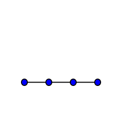
A vertex line is a sequence of vertices with a beginning and end. In any given triangulation including a vertex line, there should typically be an edge between any pair of adjacent vertices in the line.
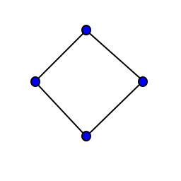
A vertex ring is a cyclic sequence of vertices. In any given triangulation including a vertex ring, there should typically be an edge between any pair of adjacent vertices in the ring, as well as an edge between the first and last vertices.
Typically, vertex lines represent edge lines, and vertex rings represent edge loops, but this is not strictly the case. For example, it is very common for an edge loop to contain a “uv seam”, where one of the vertices has to be duplicated so that the two duplicate instances can be assigned different uv coordinates. In this case, despite logically serving the role of an edge loop, the actual structure will typically be a vertex line. The resulting structure can be visualized like this:
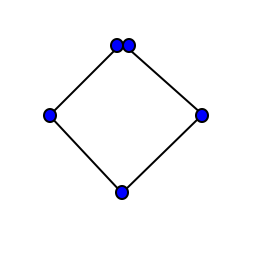
I’ve created an exaggerated gap between the start and end vertices, but in a real mesh, they would occupy the same location.
Bridges
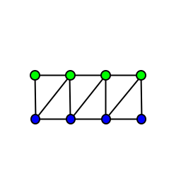
A “bridge” takes two sequences of vertices, and creates triangles spanning the gap between them in order to create a surface bridging the two lines. In the context of order-dependent triangulations, we are operating on two vertex sequences of the same length, creating edges between corresponding vertices to create a surface made of quads, and then splitting each quad into two triangles.
Bridges can be applied to either lines:
Or rings:
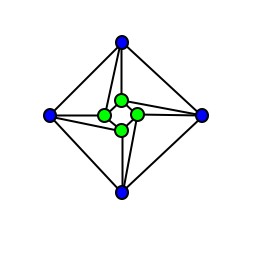
Line bridges are far more common, because even when the geometry logically “loops” around, typically there will be a UV seam somewhere on the loop that splits it into a line.
When you consider the sheer number of parts of most objects that are tubelike, you start to see how bridges alone surprisingly get you most of the way there in terms of being able to generate real geometry.
However, with real world assets, you won’t always have tidy sequences of corresponding vertices to bridge. When your vertex sequences may be of different lengths, or where the vertices may not clearly correspond to one another, you will need a more general-purpose position-dependent bridging algorithm that bridges two vertex sequences in a physically plausible way. I will be covering this kind of arbitrary bridging algorithm in a future post, along with, most likely, a number of other position-dependent triangulation algorithms.
Chaining Bridges
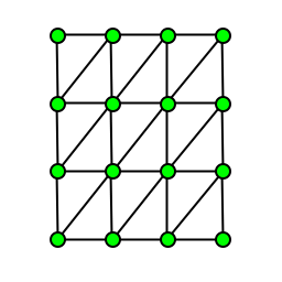
It’s very common to not just have a single bridge between two vertex sequences, but to bridge one vertex sequence to another, and then bridge that vertex sequence to a third, and bridge the third to a fourth and so on, in a long chain of bridges. This essentially joins a whole sequence of vertex sequences into a long sheet or tube.
These chained bridges can be applied to either lines:
Or rings:
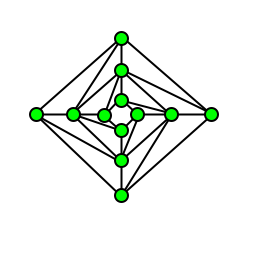
Chained bridges allow us to even more strongly take advantage of the redundancy discussed earlier. Each of these vertex sequences being bridged one-by-one have the same number of vertices. As a result, you don’t actually have to compute a start index and count individually for each vertex sequence. Instead, you can just lay out all of the vertex sequences contiguously, in the order that you plan to bridge them, then compute: the start index of the first vertex sequence, the number of vertices in each sequence, and the total number of sequences. Just as the start index and vertex count allows you to calculate an entire vertex index sequence, this set of three arguments allows you to calculate the whole sequence of starts and counts.
Domes & Spikes
The next two primitives provide different nuances on what typically looks like the same basic geometry: a sequence of vertices all being connected to a single point by “fan”. The two variants differ in their ability to support uv and normal seams.
A “dome” creates a triangle fan from a single point to the vertices in the vertex sequence. Domes are most commonly used to create a cap that has a raised, rounded center point, like, appropriately enough, a dome. However, if the point was coplanar with the other vertices, it could also be used to create a simple wheel-and-spoke cap for a polygon.
Domes can be applied to either lines:
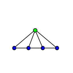
Or rings:
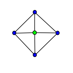
However, domes come with some inherent weaknesses. Since there is only one shared point that the entire vertex sequence connects to, that point must share the same uv coordinate and normal for every triangle of the dome. In some cases, this is not appropriate. For example, in a typical “uv sphere”, the top and bottom points of the sphere must assume different uv coordinates for each face that they are a part of. In a typical cone, all of the faces directly connecting to the point at the end of the cone need to have different normals.
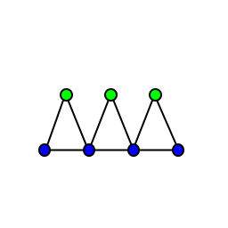
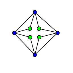
In these situations, we can instead use a “spike”. A “spike” takes two sequences of vertices and generates a sequence of triangles where each triangle contains two adjacent vertices from the first sequence, along with the vertex from the second sequence corresponding to the first vertex in the pair of vertices from the first sequence. Visually, this looks like a spike strip.
Typically, all of the vertices in the second sequence will share the same position, but the fact that they are technically different vertices means that they can have different vertex attributes, such as their normals or uv coordinates. Spikes are used to create geometry similar to a dome that is either less rounded or that has different uv coordinates on each generated face.
Spikes can be applied to either lines:
Or rings:
One big thing that differs when working with spikes and domes as compared to bridges is how you approach inverting the winding of the generated triangulation. Since bridges are symmetrical, you can invert the winding of the resulting triangles by just swapping the vertex sequences in the parameter list. But, the parameters to domes and spikes are are asymmetrical in their functions. So, you typically need two separate methods for each, one method for each possible winding. My terminology for these two versions is as follows:
- A spike or dome is “closed” if the winding of the triangles matches the winding of the vertex sequence.
- A spike or dome is “open” if the winding of the triangles is the opposite of the winding of the vertex sequence.
This naming intuitively matches the idea that, when generating a tube-like shape, you will typically “open” with an open spike or dome, build a chain of bridges, then “close” the shape with a closed spike or dome.
With just bridges, spikes and domes, many common shapes are now within reach. For example, the common “uv sphere” can be represented as a long chained bridge in its middle section, with two spikes on either end of opposite windings.
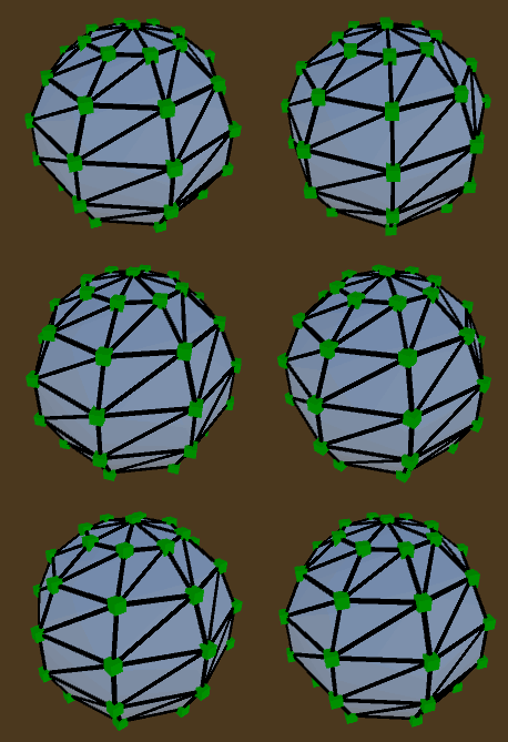
(Spikes are used rather than domes because the peak vertex on each face needs different uv coordinates, but the normals are smoothed as if the duplicate vertices at the spike were all a single vertex)
Convex Polygon Triangulation
Triangulating a polygon involves finding a collection of triangles that completely cover a polygon without overlap. The vertices of each triangle will be three of the original vertices of the polygon. Triangulating a potentially-concave polygon requires performing calculations on the vertex positions; however, if the polygon is known to be convex, it becomes a trivial order-dependent triangulation problem with a large number of possible solutions. There are a couple of specific solutions that I’ve used at various times in my own code.
Triangle Fanning
One simple way to triangulate a convex polygon is to pick a single vertex in the polygon and draw an edge from that vertex to every vertex that it is not adjacent to.
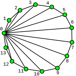
This results in a triangulation where that vertex is a member of every triangle, and resembles the “triangle fan” primitive provided by a number of graphics APIs.
Triangle Stripping
Drawing on the other common graphics API primitive, we can also triangulate a convex polygon in an order-dependent way by generating a “triangle strip” covering the polygon. In this case, we pick a vertex to start from and then traverse the perimeter in opposite directions, alternately adding a vertex from each side into the triangle strip.
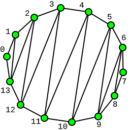
The triangle strip method has a little bit more of a balanced look to it. However, neither of these approaches really has a strong principled reason for why you would prefer it over other methods of triangulating the polygon. The third option I’ve developed for triangulating convex polygons has a little bit of an impetus behind it, and is the default algorithm I use in my own codebase.
The Approximate Max Area Algorithm
In doing some research into how polygon triangulation is handled in more professional games, I came across a description of what Emil Persson calls “The Max Area Algorithm”.
The max area algorithm operates on a few assumptions:
- When two triangles share an edge, all of the fragments along the edge may have to be redundantly rendered for both triangles, and this makes rendering the triangles take longer than if they had shared fewer fragments, even if the total number of unique fragments had been the same.
- Minimizing the total interior edge length of a polygon triangulation minimizes the redundant fragment work that the GPU has to do to render the triangles.
- Greedily picking the largest possible triangle that can be added to the triangulation at each step tends to approximate minimal interior edge length.
And from the benchmarks on the site, you can see that these assumptions hold up in practice. Coincidentally, this concern over redundant fragment rendering resulting from excessive interior edge length was recently echoed by John Carmack.
I was very interested in this idea, but, in my own asset generation code, I already have a ton of mesh generation scripts that operate by generating vertex arrays and triangle index arrays entirely independently of one another. So, a position-dependent algorithm, like the max area algorithm, is not an easy drop-in replacement for most of my own asset scripts. Instead, I started to consider if it was possible to create a “good enough” approximation that was entirely order-dependent.
The result is what you might call the “approximate max area” algorithm, a recursive algorithm that “approximately” maximizes the area of each added triangle for non-pathological convex polygons.
The approximate max area algorithm operates on two additional (handwavey) assumptions:
- Most convex polyhedra encountered in the wild have their vertices relatively evenly distributed around their perimeter in a non-pathological way.
- For non-pathological polygons, a triangle formed from three equally-spaced vertex indexes around the perimeter of the polygon will probably be pretty close in size to the largest possible triangle you could have formed.
The algorithm operates as follows:
- First form a triangle from vertex
0, vertexcount / 3and vertex2 * count / 3. This gives you one triangle and three new smaller polygons leftover by deleting that central triangle, with vertices in the ranges[0, count / 3],[count / 3, 2 * count / 3], and[2 * count / 3, count)plus0. - For each of these smaller polygons over a subsequence of the original vertex
list, we apply a recursive process:
- Create an additional triangle joining the first vertex of the subsequence, the mid point vertex of the subsequence, and the last vertex of the subsequence. This creates a new triangle and two new subsequences, from the first vertex to the midpoint, and from the midpoint to the last vertex.
- For each resulting subsequence:
- If it has exactly 3 elements, add it to the triangle list.
- If it has 4 or more elements, recurse over that subsequence.
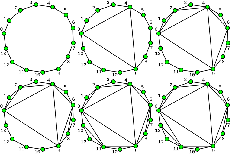
In practice, the recursive structure of the triangulation is similar to the Koch snowflake, where each new triangle that is added exposes two new exterior edges that each potentially serves as the base of another new triangle (except for the first triangle, which exposes 3 exterior edges).
For regular polygons, it seems clear that this is the same triangulation you would get from the proper max area algorithm. The resemblance can start to degrade the more lopsided the vertex distribution gets, and there can be pathological cases that cause the algorithm to generate narrow triangles. However, in these cases, any other order-dependent polygon triangulation algorithm would have almost certainly performed similarly badly. The approximate max area algorithm is probably the best you can do for the general case of triangulating a convex polygon with absolutely no position information at all, if you assume that non-pathological cases are common.
Wrapping Up
When I first started working on procedural asset generation, I took a very top-down approach of deciding on an arbitrary asset to generate, and then attempting through trial and error to figure out how to generate that asset without knowing if doing so was even possible. As I’ve spent more time over the years working on procedural asset generation code, I’ve gradually found myself shifting more to a bottom-up approach, starting from the foundational asset generation capabilities that I know my code can do well, and determining from there how to use those capabilities to generate assets. Under this new approach, order-dependent triangulations have been a consistently reliable workhorse.
Extra: Convexity-Dependent Triangulations
In between order-dependent and position-dependent triangulations, there is a secret third category that requires a tiny amount of position information, but is much less math-heavy than position-dependent triangulations. There are a number of cases where it is possible to triangulate a polygon entirely based on information about which of its vertices are convex, without considering where the vertices are located. I stumbled over these while trying to work out all of the possible early termination cases for an ear-clipping algorithm implementation. You could call these “convexity-dependent triangulations”.
Further, within convexity-dependent triangulations, there are two subcategories:
- “One shot” convexity-dependent triangulations, where, with information about the initial convexity of each vertex, you can immediately triangulate the entire polygon.
- “Incremental” convexity-dependent triangulation, where you need to iteratively clip vertices or draw edges subdividing the polygon into pieces, and then recalculate the convexity of the remaining vertices.
Within some of the descriptions below, I use terminology from the ear-clipping algorithm, so, I should briefly explain that algorithm. Every polygon has at least three convex vertices, and at least two of those convex vertices are “ears”. An ear is a convex vertex which, when you form a triangle joining that vertex with each of its adjacent vertices, the resulting triangle will not contain any of the other vertices in the polygon. “Clipping” a vertex, involves taking this triangle and adding it to the triangulation, then removing the vertex from the polygon, leaving an edge between its former neighbors in its place. In the special cases described below, we will be clipping vertices, but we will be determining whether or not they are ears through alternative convexity-based methods.
N-Gons with Exactly Zero Concave Vertices
If a polygon has exactly zero concave vertices, then the polygon is convex, so we can immediately use an order-dependent convex polygon triangulation algorithm. So, this is a one-shot convexity-dependent triangulation.
N-Gons with Exactly One Concave Vertex
If a polygon has exactly one concave vertex, we can always draw edges from that vertex to every vertex it is not adjacent to. This creates a triangle fan, triangulating the entire polygon. So, this case is also a one-shot convexity-dependent triangulation.
N-Gons with Only Contiguous Concave Vertices
We can incrementally triangulate any N-Gon which has any number of concave vertices as long as all of those vertices are contiguous, by taking advantage of a few key observations:
- If all of the concave vertices in a polygon are contiguous, the convex vertices on either side of that concave vertex sequence must always be ears, so triangles can always be clipped from those vertices.
- A concave vertex can become convex after one of its neighbors is clipped, but a convex vertex can never become concave after a neighbor is clipped.
So, our incremental algorithm becomes:
- Identify the sequence of contiguous concave vertices and the two clippable convex vertices at either end.
- Clip either one of the two convex vertices.
- Reevaluate the convexity of the concave vertex adjacent to the clipped vertex. If it has become convex, then it is now the new clippable convex vertex on that side of the sequence. Otherwise, the vertex that is now adjacent to it post-clip is the new clippable convex vertex on that side of the sequence.
- Repeat from step 2 until the triangulation is complete.
N-Gons with Exactly Two Non-Contiguous Concave Vertices
If a polygon has exactly two non-contiguous concave vertices, then it is always possible to triangulate it with incremental convexity information. The only required observation is that when a polygon has exactly two concave non-adjacent vertices, an edge connecting those two vertices will always lie entirely within the polygon. So, you can draw this edge to split the polygon into two separate polygons.
The resulting pair of polygons will collectively have, at most, two concave vertices, and whatever concave vertices exist in either of the resulting polygons will be in a contiguous group, so you can apply the contiguous concave vertex rule from above.
3-Gons
A 3-gon is, by definition, already a triangle, so we can one-shot a 3-gon without even checking the convexity of its vertices.
4-Gons
As stated in our earlier rule, every polygon must have at least 3 convex vertices. This means that a 4-gon can have either zero or one concave vertices. Both of these cases fall under our special case rules for one-shot triangulating a polygon.
In terms of implementing this triangulation, we can actually get away with checking the convexity of a smaller subset of the vertices. We just have to check any two opposite vertices (at an offset of 2 in the vertex sequence).
- If one of the two is concave, then we have found the only concave vertex, and we can apply our rule for polygons with exactly one concave vertex. In this case, that would just involve drawing a single edge between the two vertices that we checked, clipping the other two vertices.
- If neither is concave, then we can just assume that one of the other two vertices might be concave and apply the same rule. Whether either of them are concave or not, this will always result in a valid triangulation.
5-Gons
5-gons can have, at most, 2 concave vertices. This still causes 5-gons to fall within our special cases, but it potentially spills into our “incremental” cases of either multiple contiguous concave vertices, or two non-contiguous concave vertices. So, in the worst case scenario, triangulating a 5-gon based on convexity is an incremental algorithm.
In terms of implementing this triangulation, we can start off by checking the convexity of three vertices that are not all contiguous.
- If the checked vertices are all convex, then we can clip the checked vertex that is not contiguous to the other two, and then apply the 4-gon algorithm to the remaining vertices.
- If two of the checked vertices are concave, then we can apply the appropriate special case based on whether they are contiguous or non-contiguous.
- If one of the checked vertices is concave, then we handle it based on whether
it is one of the pair of contiguous checked vertices, or the lone
non-contiguous checked vertex.
- If one of the pair of contiguous checked vertices is concave, then we can always clip the other vertex in the pair. This leaves us with a 4-gon.
- If the lone non-contiguous checked vertex is concave, we have to check one of the remaining unchecked vertices. If it is convex, we can clip it; otherwise we can clip the other one. In either case, we are left with a 4-gon.
Failure of the General Case of 6-Gons
6-Gons are the first instance where we can construct an example where multiple polygons that must be triangulated differently have the same vertex convexity pattern, meaning that, in the general case, 6-gons cannot be triangulated with convexity information alone.
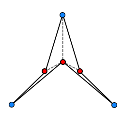
Here, the concave vertices are colored red, and the convex vertices are colored blue. There is only one valid triangulation of this polygon, which is drawn with dotted lines.
In this case, the convexity pattern is a symmetrical alternation of: convex, concave, convex, concave, convex, concave. However, the required triangulation is asymmetrical, as only two of the three convex vertices can be clipped. It’s not possible to deduce which two these are given only the convexity information, so generating the triangulation is impossible.
Higher order polygons also have this same issue, as you could extend this shape by adding additional convex vertices arbitrarily close to the existing convex vertices. Since it wouldn’t be possible to deduce whether the new vertices were added adjacent to a clippable vertex or not, these added vertices would not aid in triangulating the core underlying 6-gon.
Other Convexity-Dependent Rules
I am not personally aware of any other special cases or solutions for convexity-dependent triangulations. If you happen to know of or discover one, let me know, and I can add it here and credit you for it.